
As the season gets underway, I’ve been thinking about the importance of coordinators and how their tendencies can be used against them. Past investigations into this topic have shown that certain coordinators have a high pass rate over expected and that this is mostly sticky throughout the season. But nobody has attempted to incorporate who the coordinator is in their pass probability models. Thus, I decided to fill this gap and attempt to build an xPass model with coordinator mixed effects.
In this post I;
- Use Python to build a tree boosted mixed effects model that provides a probability of pass for any given scenario
- Examine coordinator pass probabilities under various scenarios
Data
As outlined in my previous post, I scraped PFR for their coordinator level data and output it into a format that can be quickly joined to PBB data. I loaded this data into Python and only selected the last 6 years of data (otherwise my computer will run very very slow). An important aspect of my analysis is that I am considering each coordinator year as its own group, meaning the model will view coordinator 2019 as different than coordinator 2020. My reasoning is that tendencies can change between years because of personnel so it is more effective to assign situational pass probabilites year by year and then compare those charts. Ideally, there is a way to weight more recent coordinator observations so that the predictions are not skewed by old seasons. This is something to explore in the future though.
#Load in packages
from gpboost.engine import train
import pandas as pd
import numpy as np
import gpboost as gpb
from sklearn.model_selection import train_test_split
import matplotlib
from sklearn.model_selection import GroupShuffleSplit

#change options and set seed
pd.set_option("display.max_rows", None, "display.max_columns", None)
np.random.seed(59)

#load in data & check
pbp_data = pd.read_csv("C:/Users/Joe/Desktop/Coordinator_NFL_Final.csv")
pbp_data.head(5)
Issues and Solutions
Incorporating categorical variables into a random forest model can be approached from multiple angles, one could one hot encode how ever many coordinators into the data or just build the random forest model and insert a mixed effect for coordinators after. Both approaches are suboptimal though and I saught out a solution that combines random forests wtih mixed effects. I found the GPboost package as a result, the package combines tree-boosting and mixed effects to create one model. I’ve never seen this method used in the sports space to my knowledge so this required a fair amount of trial and error on my part (especially since I am still new to Python). Nevertheless, I powered through and learned a lot about Python along the way.
With one issue out of the way, I found another new problem. A traditional train test split would not be a good idea for this mixed effect model because we would run the risk of overrepresenting certain coordinators or underrepresenting in the train or test sets. And because we are interested in every coordinator, we have to make sure each one has an equal proportion of data in the train and test sets we will be using. So, I wrote a simple loop that takes 70% of each coordinators season data and adds it to a train dataframe while the remaining proportion is put into a test set.
#Select our target and variables of interest

modeling_data = pbp_data[["yardline_100",
                          "qtr",
                          "half_seconds_remaining",
                          "ydstogo",
                          "down",
                          "shotgun",
                          "score_differential",
                          "posteam_timeouts_remaining",
                          "defteam_timeouts_remaining",
                          "wp",
                          "O_Coordinator",
                          "pass"]]

# Train test method

train_final  = pd.DataFrame()
test_final   = pd.DataFrame()
Coordinators = modeling_data['O_Coordinator'].unique()
length = len(Coordinators)
for x in range(length):
    Coordinator_X = Coordinators[x]
    Data_Filtered = modeling_data[modeling_data['O_Coordinator'] == Coordinator_X]
    train, test   = train_test_split(Data_Filtered, test_size= .3, random_state=94)
    train_final   = train_final.append(train)
    test_final    = test_final.append(test)
Building the Model
Now we can move onto training our model and tuning the hyperparameters. The first thing we want to do is specify our likelihood function and then define what variable should be used in the mixed model. This is done via the GPModel function in python. I also create the GPModel dataset for the fixed effects portion and make the pass variable our target. Note that I include the shotgun variable in my model. I considered not including it as the NFLFastR xPass model does not but I got worse results when not including Shotgun.
# Set likelihood function to use
likelihood = "bernoulli_logit"

# Define random effects model (OC) & insert the likelihood
gp_model = gpb.GPModel(group_data=train_final[['O_Coordinator']], likelihood=likelihood)

# Create dataset for gpb.train
data_train = gpb.Dataset(data=train_final[[
     "yardline_100",
     "qtr",
     "half_seconds_remaining",
     "ydstogo",
     "down",
     "shotgun",
     "score_differential",
     "posteam_timeouts_remaining",
     "defteam_timeouts_remaining",
     "wp"]],
     label=train_final['pass']) #pass is our target so we set that as the label
Next, we can specify our objective and parameters. I opted to use the random search function in the GPBoost package which allowed me to tune hyperparameters. I started with some general hyperparamter values to try and the model combines these values at random to test their performance. I also made a few changes to the grid search function and only tried 10 rounds of random combos because I have a bad computer and I also use the training data for 5 fold cross validation. I further am using log loss as the eval metric.
# Set model parameters
params = {'objective': 'binary',
          'verbose': 0,
          'num_leaves': 2**10 }

# Grid for model to search through
param_grid = {'learning_rate': [0.5,0.1,0.05,0.01,.2], #eta
                'max_depth': [1,3,5,10,20], #max_depth
                'min_sum_hessian_in_leaf': [2,8,15,20,25,40], #min_child_weight
                'bagging_fraction': [.1,.25,.35,.55,.75], #subsample
                'feature_fraction': [.1,.25,.35,.55,.75]} #colsample_bytree

# Grid search
opt_params = gpb.grid_search_tune_parameters(param_grid=param_grid,
                                             params=params,
                                             num_try_random=10, #40 rounds
                                             nfold=5, #5 fold cross validation
                                             gp_model=gp_model, #random effects
                                             use_gp_model_for_validation=True,
                                             train_set=data_train, #training set
                                             verbose_eval=1,
                                             num_boost_round=1000,
                                             early_stopping_rounds=25, #stop at 25 if no improvement
                                             seed=1,
                                             metrics='binary_logloss') #log loss as eval metric

# Print best options
print("Best number of iterations: " + str(opt_params['best_iter']))
print("Best score: " + str(opt_params['best_score']))
print("Best parameters: " + str(opt_params['best_params']))
Great! It appears the model is honing in on a learning rate in the mid .2’s and a max depth around 5. In response, I will change my param grid to try to fine tune the hyperparameters. I set some new parameters in this range and re-run the model below.
# Reevaluate parameters
param_grid = {'learning_rate': [.24,.25,.26],
                'max_depth': [4,5,6],
                'min_sum_hessian_in_leaf': [36,38,40],
                'bagging_fraction': [.3,.35,.4],
                'feature_fraction': [.22,.25,.27]}

# Same grid search with new parameters
opt_params = gpb.grid_search_tune_parameters(param_grid=param_grid,
                                             params=params,
                                             num_try_random=15,
                                             nfold=5,
                                             gp_model=gp_model,
                                             use_gp_model_for_validation=True,
                                             train_set=data_train,
                                             verbose_eval=1,
                                             num_boost_round=1000,
                                             early_stopping_rounds=15,
                                             seed=1,
                                             metrics='binary_logloss')
print("Best number of iterations: " + str(opt_params['best_iter']))
print("Best score: " + str(opt_params['best_score']))
print("Best parameters: " + str(opt_params['best_params']))
I won’t pain you with the fine tuning because it is just me trying smaller numbers to hone in on the best combo. Eventually, the model returned a:
- learning_rate: 0.26
- max_depth: 6
- min_sum_hessian_in_leaf: 38
- bagging_fraction: 0.35
- feature_fraction: 0.25
- boosting rounds: 999
We can now train the model with these parameters and check our importance plot.
# Train with best parameters
params = { 'objective': 'binary',
            'learning_rate': 0.26,
            'max_depth': 6,
            'min_sum_hessian_in_leaf': 38,
            'bagging_fraction': 0.35,
            'feature_fraction': 0.25,
            'verbose': 0 }

# Train GPBoost model
bst = gpb.train(params=params,
                train_set=data_train,
                gp_model=gp_model,
                num_boost_round=999,
                valid_sets=data_train)

# Estimated random effects model
gp_model.summary()

# Check importance
gpb.plot_importance(bst)
Nothing too surprising here. We can now proceed by fitting our model to the test data and checking model calibration.
# Define random effects model (OC)
group_test = test_final[["O_Coordinator"]]

# Create dataset for gpb.train
data_test = test_final[[
     "yardline_100",
     "qtr",
     "half_seconds_remaining",
     "ydstogo",
     "down",
     "shotgun",
     "score_differential",
     "posteam_timeouts_remaining",
     "defteam_timeouts_remaining",
     "wp"]]

# Make predictions on the test set
pred = bst.predict(data=data_test,
                    group_data_pred= group_test,
                    raw_score=False)

# Add predictions to dataframe of variables
Probs = pd.DataFrame(data = pred['response_mean'])
test_final.reset_index(drop=True, inplace=True)
Probs.reset_index(drop=True, inplace=True)
df = pd.concat( [test_final, Probs], axis=1)
df.to_excel('test.xlsx')

#save model
bst.save_model('xPass_model.json')

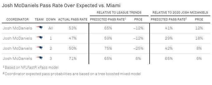
I created this calibration plot in R as I am still not the most familiar with Python plotting yet. Nevertheless, it looks like our model is well calibrated and ready for deployment. One thing we can do is observe how much more pass happy or run heavy a team is in 2021 relative to their 2020 counterpart. Not all coordinators returned in 2021 so some teams are represented by a different coordinator. One coordinator of interest to me is Josh McDaniels, we can fit week 1 against Miami with the model to observe his pass tendency relative to 2020.
#examine some situations
first_q_situations = pd.read_csv("C:/Users/Joe/Desktop/Coordinator_NFL_Final_try.csv")
first_q_situations["O_Coordinator"] = 'Josh McDaniels_2020'

OC = first_q_situations[["O_Coordinator"]]

# Create dataset for gpb.train
situations_variables = first_q_situations[[
     "yardline_100",
     "qtr",
     "half_seconds_remaining",
     "ydstogo",
     "down",
     "shotgun",
     "score_differential",
     "posteam_timeouts_remaining",
     "defteam_timeouts_remaining",
     "wp"]]

# Make predictions on the test set
pred = bst.predict(data=situations_variables,
                    group_data_pred= OC,
                    raw_score=False)

# Add predictions to dataframe of variables
Probs = pd.DataFrame(data = pred['response_mean'])
situations_variables.reset_index(drop=True, inplace=True)
Probs.reset_index(drop=True, inplace=True)
df = pd.concat( [situations_variables, Probs], axis=1)
df.to_excel('Joshy.xlsx')
Now we can put the data into a table (done in R because tables in Python are not fun) and see that
- Josh McDaniels called a conservative game relative to what the league would have done in the game situations he was presented with
- He was more aggressive than last year in terms of passing rate, which shows how conservative he was in 2020.
This is the advantage of having a coordinator adjusted model, we can see how an OC may be changing their style or how personel is influencing their play calls.
We can do this for the rests of the league as well, some teams have different OC’s so I just used whomever was the 2020 OC as their previous season ref point. A few things that stand out/should be noted.
- I removed post-Dak injury games which dramatically improved the predictive power of Kellen Moore’s 2020 season on week 1 vs Tampa Bay.
- Washington fell into the 2 high safety Brandon Staley trap and ran too much (although some can be attributed to the Fitz injury).
- Buffalo passed so much last year that any return to normalcy would appear dramatic.
