We are all aware of team tendencies in the NFL and how certain ones are more pass heavy than others. What is not well researched is how this may vary on the coordinator level and if certain OC’s have tendencies that can be picked up on. In this post, I scrape PFR for coordinator data (OC & DC), clean the data, and develop a simple model with the OC as a random effect. I then analyze how each OC increases the probability of passing on 1st & 10.
Scraping PFR
This process was very similar to my previous post regarding injury scraping on PFR. I followed the same process of constructing URLs for each page and combining them with years to get a list of URLs to scrape through. I won’t delve into that again and instead will move onto the scraping function. The function is interested in the coaches info you can see at the top of the team page. My process can be found below but the basic idea was that all of the coordinator info is located in the same node. I scrape that node, use regex to search for defensive or offensive coordinator, and then add that to a dataframe. I also scrape important id info such as season and team so that the data can be added to play by play data. Once this is done, I clean the data so that it is easily understood.
coordinator_scraper <- function(urls) {

url   <- read_html(urls)

A <- url %>%
  html_nodes("p") %>%
        html_text() %>%
  as.data.frame() %>%
  rename("O_Coord" = ".") %>%
  filter(across(O_Coord, ~ grepl('Offensive Coordinator', .)))
A <- ifelse(length(A$O_Coord) < 1,
       url %>%
       html_nodes("p") %>%
       html_text() %>%
       as.data.frame() %>%
       rename("O_Coord" = ".") %>%
       filter(across(O_Coord, ~ grepl('Coach:', .))) ,
       A) %>%
  as.data.frame()
colnames(A)[1] <- "O_Coord"
B <- url %>%
  html_nodes("p") %>%
        html_text() %>%
  as.data.frame() %>%
  rename("D_Coord" = ".") %>%
  filter(across(D_Coord, ~ grepl('Defensive Coordinator', .)))
B <- ifelse(length(B$D_Coord) < 1,
       url %>%
       html_nodes("p") %>%
       html_text() %>%
       as.data.frame() %>%
       rename("D_Coord" = ".") %>%
       filter(across(D_Coord, ~ grepl('Coach:', .))) ,
       B) %>%
  as.data.frame()
colnames(B)[1] <- "D_Coord"
C <-url %>%
  html_nodes("p") %>%
        html_text() %>%
  as.data.frame() %>%
  rename("Team" = ".") %>%
  filter(across(Team, ~ grepl('Franchise', .)))
D <-url %>%
  html_nodes("p") %>%
        html_text() %>%
  as.data.frame() %>%
  rename("Season" = ".") %>%
  filter(across(Season, ~ grepl('Statistics', .)))
data <- cbind(A,B,C, D)
return(data)
}
###Create empty data frame to store data
empty <- data.frame()
###Create loop that will go through our urls and return injuryies
for (x in url_list) {
output <- coordinator_scraper(x)
empty <- rbind(empty, output)
}

Cleaned_Data <- empty

#remove uneeded data
Cleaned_Data$O_Coord <- gsub("Offensive Coordinator: ","", Cleaned_Data$O_Coord)
Cleaned_Data$O_Coord <- gsub("Coach: \n ","", Cleaned_Data$O_Coord)
Cleaned_Data$D_Coord <- gsub("Defensive Coordinator: ","", Cleaned_Data$D_Coord)
Cleaned_Data$D_Coord <- gsub("Coach: \n ","", Cleaned_Data$D_Coord)
Cleaned_Data$Team    <- gsub("Franchise Pages","", Cleaned_Data$Team)

#clean season column
Cleaned_Data$Season <- str_sub(Cleaned_Data$Season, 1, 4)
Cleaned_Data$Season <- as.numeric(Cleaned_Data$Season)

#clean coordinator columns that have records because HC is the coordinator
Cleaned_Data$O_Coord <- gsub("[[:digit:]]+","",Cleaned_Data$O_Coord)
Cleaned_Data$O_Coord <- gsub("(--)","",Cleaned_Data$O_Coord)
Cleaned_Data$O_Coord <- gsub(paste(c("[(]", "[)]"), collapse = "|"), "", Cleaned_Data$O_Coord)
Cleaned_Data$D_Coord <- gsub("[[:digit:]]+","",Cleaned_Data$D_Coord)
Cleaned_Data$D_Coord <- gsub("--","",Cleaned_Data$D_Coord)
Cleaned_Data$D_Coord <- gsub(paste(c("[(]", "[)]"), collapse = "|"), "", Cleaned_Data$D_Coord)
Cleaned_Data <- Cleaned_Data %>%
  rename("Coord_O" = O_Coord) %>%
  rename("Coord_D" = D_Coord)

#Make data long for merging with PBP
Cleaned_Data <- Cleaned_Data %>%
 pivot_longer(
   cols = starts_with("Coord"),
   names_to = "Coord",
   names_prefix = "Season",
   values_to = "Coordinator",
   values_drop_na = TRUE
 ) %>%
  rename("Side_of_Ball" = "Coord") %>%
  mutate(Side_of_Ball = ifelse(Side_of_Ball == "Coord_O", "Offense", "Defense"))
This was much easier than scraping PFR for injury related data. I then added the data into the play by play data and prepared for modeling.
GAM Model
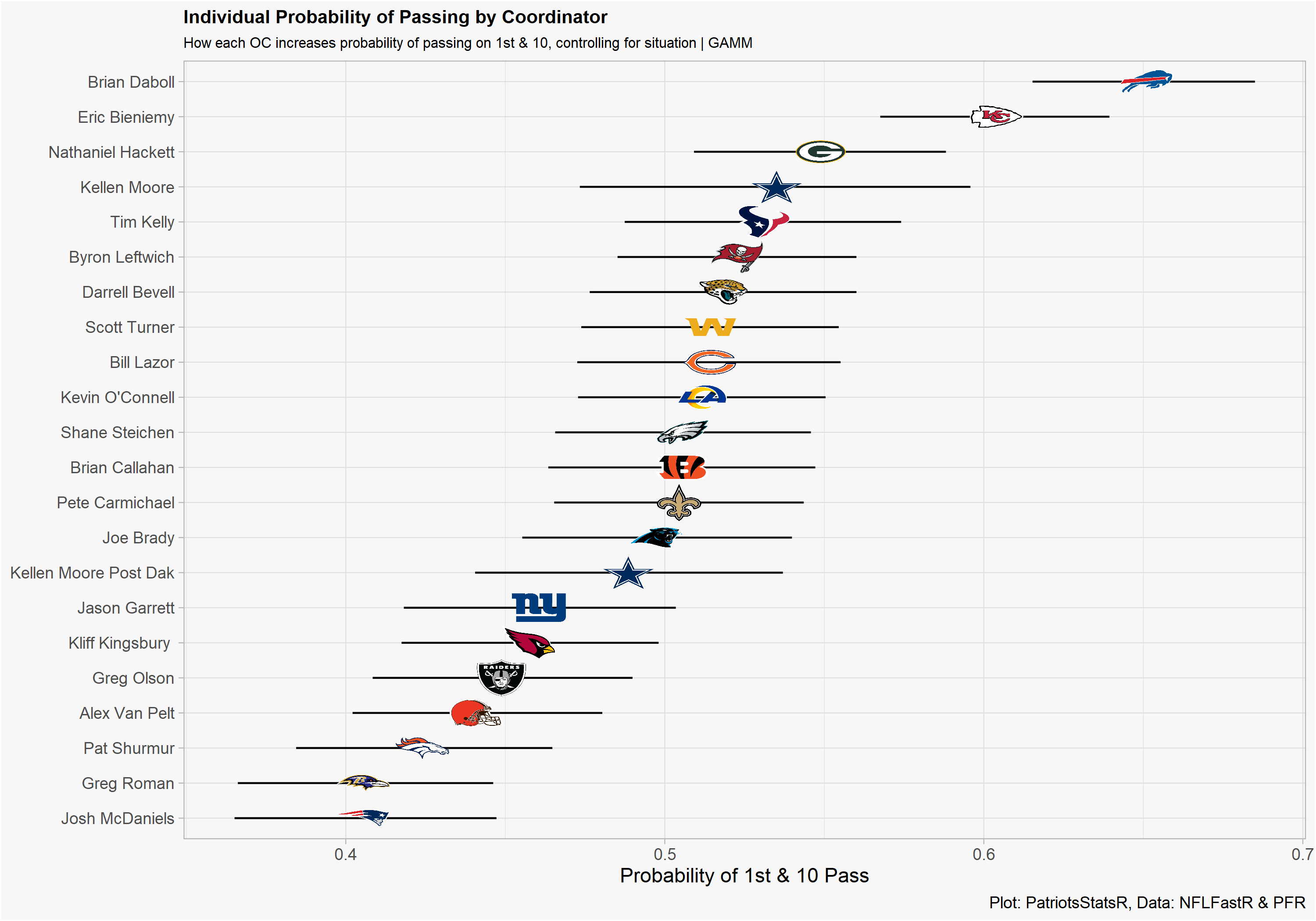
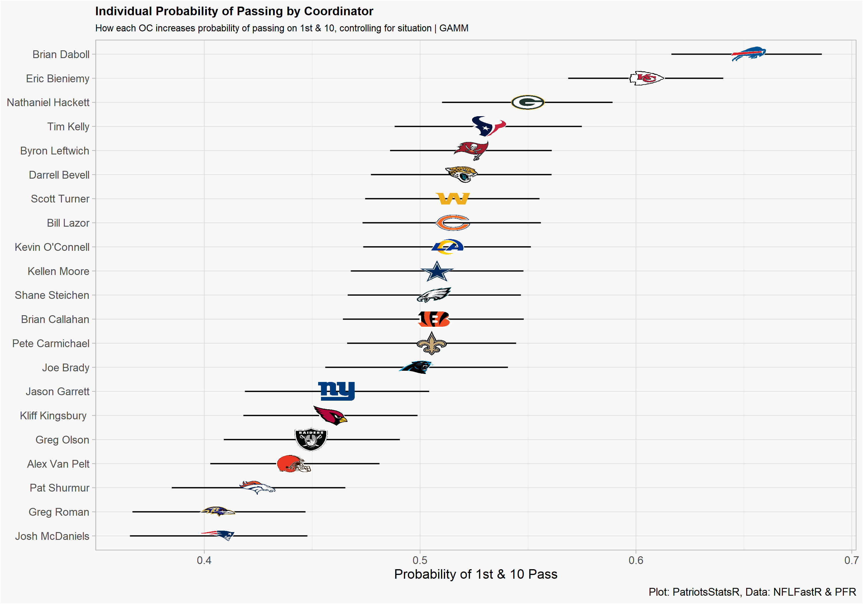
This topic can be applied to any situation but for this post I chose to focus on a very common situation: 1st & 10. My objective was to use a mixed effects GAM model to measure the individual effect on pass probability that each OC has. The higher the intercept, the higher the probability of a pass taking place just because of who the OC is. In the model, I am only interested in OC’s who will be calling plays in 2021 so I filtered my dataframe for those individuals.
gam_model <- gamm4(
    play_type ~
    ydstogo +
    yardline_100 +
    down +
    wp +
    half_seconds_remaining +
    score_differential +
    qtr,
  random = ~ (1 | O_Coordinator),
  data = pbp_data,
  nAGQ = 0,
  control = glmerControl(optimizer = "nloptwrap"),
  family = binomial(link = "logit")
)

    #Retrieve estimates and standard errors
  est <- broom.mixed::tidy(gam_model$mer, effects = "ran_vals") %>%
    dplyr::rename("Coord" = "level") %>%
    dplyr::filter(term == "(Intercept)")

  # Function to convert logit to prob
  logit2prob <- function(logit) {
    odds <- exp(logit)
    prob <- odds / (1 + odds)
    return(prob)
  }

  # Prepare data for plot
  plot <- merge(est, names, by = "Coord", all.x = T, no.dups = T) %>%
    arrange(estimate) %>%
    mutate(
      lci = estimate - 1.96 * std.error,
      uci = estimate + 1.96 * std.error,
      prob = logit2prob(estimate),
      prob_uci = logit2prob(uci),
      prob_lci = logit2prob(lci)
    )


  #merge in team logos
  plot  <- plot %>%
    left_join(nflfastR::teams_colors_logos, by = c("posteam" = "team_abbr"))

  return(plot)
Now we can plot the data.
One bias in this model is that we are not accounting for who the QB is. For example, before Dak was injured Kellen Moore was among the highest individual probability estimates in our model. When Dak was hurt, Moore obviously passed less and his estimate fell.