Bayesian Updating of College Football Completion Percentage

Recently I have been reading Statistical Rethinking along with Introduction to Empirical Bayes: Examples from Baseball Statistics. Both discuss Bayesian techniques in R, the latter discussing Bayes in the context of baseball and batting averages. This got me thinking of binary outcomes that I could measure in football and how to apply some of the techniques outlined by the author. One topic that quickly came to mind was completion percentage in college football (as CFB doesn’t have CPOE data I figured this would be more applicable than NFL). In this post, I establish a framework for evaluating CFB QB completion percentage with Bayes and informative priors that take advantage of recruit ranks.

##Quick Background on Bayes in this Analysis

Bayesian techniques are not new but they are also not used nearly as often as frequentist methods in public analysis, thus they are not always well understood. In its simplest form, Bayes works by 1. evaluating your prior beliefs on a topic, 2. evaluating the evidence, and 3. then returning a credible interval of what the true value is given what we have seen and what we knew before seeing the evidence. This can be best understood when applied to QB CP%:

1. Prior: Based on how 5 star recruit QB’s have performed in the past, we expect 5 star QB x to have a career CP% somewhere in the range of 45% to 70%.
2. Evidence: We see QB x throw 400 passes and only complete 200 (50%).
3. Bayes Evaluation: Considering the prior and evidence, our estimate of QB x’s true CP% shifts to a new range of 40% to 55% (purely hypothetical). This happens because the evidence is strong enough to essentially discard our prior that QB x had a high ceiling. As the QB throws more passes, his range will shrink.

Data & Cleaning

I used the CFB Fast R API to obtain CFB QB data from 2014 to 2020. In addition, I loaded in CFB recruiting class data from the CFB Data API for the years 2000 to 2020. Not all of these years are needed but I wanted to ensure that any QB who played in our play by play dataset was captured by the recruiting data. I then filtered for dual threat and pro players (both QBs) and merged recruit info with pbp data. Below is a code snippet of the data call, full cleaning can be found in my GitHub but it primarily involves joining the data and making sure there are no issues.

pbp <- data.frame() #blank frame
#Loop
for (x in 2014:2020) {
  progressr::with_progress({
  future::plan("multisession")
  qb_perf <- cfbfastR::load_cfb_pbp(x)
  qb_perf <- qb_perf %>%
  filter(pass == 1) %>%
  dplyr::select(passer_player_name,
         year,
         week,
         pos_team,
         def_pos_team,
         EPA, 
         pass,
         game_id,
         id_play,
         game_play_number, 
         completion,
         pass_attempt)
  pbp <- rbind(pbp, qb_perf)
  
  })
}
qb_ratings <- data.frame() #blank data frame for merging
for (x in 2000:2020) {
  PRO  <- cfbd_recruiting_player(x, position = "PRO")
  DUAL <- cfbd_recruiting_player(x, position = "DUAL")
  qb_ratings <- rbind(qb_ratings, PRO, DUAL)
}

Exploring Predictors of QB Completion Percentage

Recruiting Rankings

When evaluating CFB QB’s, we always have access to some prior information regarding their ability. This can be actual in game performance or it can be their prestige, aka their recruiting rating. There are a few different metrics by which CFB players are graded (stars, composite ranking, overall class rank) that we can use to give our model some guidance on what to expect from a QB. For context, one important aspect of Bayesian analysis is priors and how they can guide a model in the absence of much data. A prior essentially says that given player x’s recruiting ranking, what are the range of outcomes related to a variable of interest (in our case completion percentage). This is a very valuable tool for determining the possible outcomes for a QB who we don’t have much information on (such as a freshman or redshirt). Back to CFB recruit grades, we first must determine which of the mentioned variables are most predictive of a CFB QB’s completion percentage. Below, I evaluate the correlation between each metric and career completion percentage.

All metrics are close to each other in terms of correlation. Thus, I chose to use the composite rating (0-100 scale) because of the added layer of granularity relative to stars. We can visualize the relationship between composite rating and CP% with a smoothing spline below.

Number of Throws

As mentioned in Empirical Bayes: Examples from Baseball Statistics, one confounder in sports is how many opportunities a player gets. In our case, a QB who is bad will get less opportunities to throw the ball than a QB who is good (this is obvious). The reason this is an issue is because of the plot below, our estimates would be biased and we would shrink players who have low attempts too much towards the overall league average and overestimate CP%. We can account for this by also adding the numbers of attempts to our model.

Years of Experience

In a similar vain, QB years of experience can also serve as a valuable prior for predicting QB CP%. The visual below displays this relationship and shows that QB experience is correlated with CP%. This is important because of QBs who may have reshirted their freshman year (or QBs who threw very few passes their freshman year), we know QBs in this situation spent the season learning and this should lead into better QB play their sophomore year. If we only accounted for QB composite ranking then this effect would be missed and the prior for a sophomore 5 star QB would be the same as a freshman 5 star QB. A recent example of this is Mac Jones (not 5 stars). He was not redshirted but only threw 13 attempts in his freshman year. In the model, Mac’s range of possible outcomes increases because history says that QB CP% rises with their level of experience. Very important caveat here on survivorship bias, good QBs are allowed to play more and therefore will have more years of experience. This is baked into the model and i would argue it is fine because 1. a coach is unlikely to willingly start a QB who redshirted or hardly played their freshman if they are obviously terrible (so we should assume the QB has some potential) and 2. it has been shown that when older players play younger players in CFB that the older players perform better.

Model Fitting

Now we can fit our model, I used a beta prior and a GAM. The simplest way to explain the model is that every QB has a unique prior of how we should expect them to perform based on their composite rating, years of experience, and number of attempts. If a QB has very few throws then these factors will largely determine their range of outcome estimate. If a QB has a large body of work then their range of outcomes is largely determined by what they have done and the prior is mostly out of play.

##Data to fit
QB_Grouped <- QB_Data %>%
  mutate(Years_Since_Entry = ifelse(Season == class, 0, 
                             ifelse(Season == class+1, 1,
                             ifelse(Season == class+2, 2,
                             ifelse(Season == class+3, 3,
                             ifelse(Season == class+4, 4, 5)))))) %>%
  group_by(id, name, rating, Years_Since_Entry) %>%
  summarize(throws      = n(),
            cp          = sum(completion) / sum(pass_attempt),
            completions = sum(completion),
            attempts    = sum(pass_attempt)) %>%
  ungroup()
##fit gam lss
fit <- gamlss(cbind(completions, attempts - completions) ~ 0 + log(attempts) + rating + ns(Years_Since_Entry, df = 4),
              data = QB_Grouped,
              family = BB(mu.link = "identity"))
tidy(fit)
#fit model to data
mu    <- fitted(fit, parameter = "mu")
sigma <- fitted(fit, parameter = "sigma")
career_eb_wCP <- QB_Grouped %>%
  dplyr::select(name, id, completions, attempts, rating, Years_Since_Entry) %>%
  mutate(mu = mu,
         alpha0 = mu / sigma,
         beta0 = (1 - mu) / sigma,
         alpha1 = alpha0 + completions,
         beta1 = beta0 + attempts - completions,
         new_eb = alpha1 / (alpha1 + beta1),
         low = qbeta(.025, alpha1, beta1),
                high = qbeta(.975, alpha1, beta1)) 

Great! Now we have our model and can apply it to our data via Bayesian updating. We are curious about how a QB’s range of possible outcomes changed throughout their career after each throw. I do this by creating a function that calculates at each throw a few factors:

• Years of experience
• Rolling cumulative attempts and completions

At each point the model returns the credible interval for the QB and where we should expect their CP% to lie.

QB_Graphing_Function <- function(QB_Name, color_code) {
a <- QB_Data %>%
  mutate(Years_Since_Entry = ifelse(Season   == class, 0, 
                             ifelse(Season == class+1, 1,
                             ifelse(Season == class+2, 2,
                             ifelse(Season == class+3, 3,
                             ifelse(Season == class+4, 4, 5)))))) %>%
  filter(name == QB_Name) %>%
  arrange(start_date, game_play_number) %>%
  within(acc_sum_cp <- cumsum(completion)) %>%
  within(acc_sum_at <- cumsum(pass_attempt))
b <- career_eb_wCP %>%
  arrange(desc(new_eb)) %>%
  filter(  name == QB_Name  ) %>%
  dplyr::select(-new_eb,
         -low,
         -high)
         
return(merge(a,b, by = c("name", "id", "Years_Since_Entry")) %>%
  mutate(alpha1 = alpha0 + acc_sum_cp,
         beta1 = beta0 + acc_sum_at - acc_sum_cp,
         new_eb = alpha1 / (alpha1 + beta1),
         low = qbeta(.025, alpha1, beta1),
                high = qbeta(.975, alpha1, beta1))
                
                }

Analysis & Plots

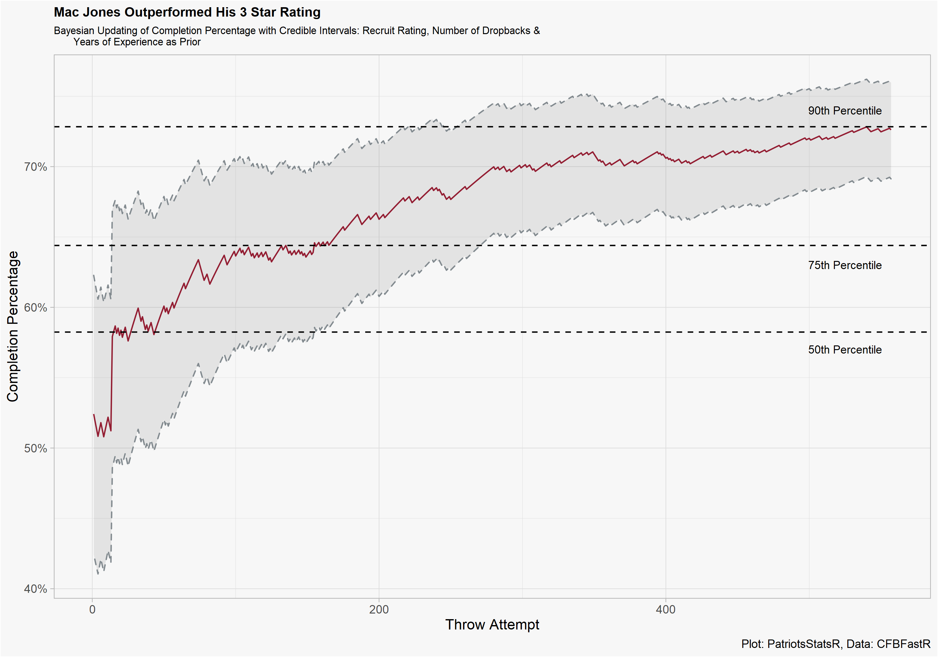
Now the interesting part, we can observe new Patriots QB Mac Jones and his range of CP% outcomes according to the model. A quick few notes on graphic interpretation:

• The grey area represents what Mac Jones “true” CP% is at each given throw. As he accumulates more attempts this grey area shrinks because the model is more sure of his CP%.
• The big jump at the start of the graphic is when Jones became a sophomore QB. Because there was virtually no evidence of Jones CP%, the prior on experience has a large effect causing his estimate to be much higher.
• This should not be interpreted as “we should sit QB x their freshman year because sophomore QBs have a higher CP%”. There was still a very wide range of outcomes for Mac entering his sophomore year, from bad to top 25 percentile.
• I would argue that the model not putting Mac’s final CP% in the credible interval is a sign of validity. Do you really want a model to predict a 95th percentile outcome on a 3 star QB with no evidence?

A good comp for how this would work with a highly ranked QB is Trevor Lawrence. He provides some context on the range of outcomes for a very high composite ranking freshman, how the model updates to reflect his performance, and how there is not much of an effect related to years of experience because he played right away.

---